Collision World Representation
World Representation
cuRobo represents the world with an instance of curobo.geom.types.WorldConfig which
can store world objects as primitives, meshes, and depth images using nvblox or voxelization.
cuRobo has GPU accelerated functions for collision queries with cuboids, meshes, nvblox maps, and
euclidean signed distance voxel grids. Other primitive types can be approximated to a cuboid or a
mesh using helper functions described later in this page. An overview of the world representation
and collision checkers is illustrated below.
We will look at some examples in python. First, we will load a world that contains one object of each type,
from curobo.geom.types import WorldConfig, Cuboid, Mesh, Capsule, Cylinder, Sphere
from curobo.util_file import get_assets_path, join_path

obstacle_1 = Cuboid(
     name="cube_1",
     pose=[0.0, 0.0, 0.0, 0.043, -0.471, 0.284, 0.834],
     dims=[0.2, 1.0, 0.2],
     color=[0.8, 0.0, 0.0, 1.0],
 )

# describe a mesh obstacle
# import a mesh file:

mesh_file = join_path(get_assets_path(), "scene/nvblox/srl_ur10_bins.obj")

obstacle_2 = Mesh(
   name="mesh_1",
   pose=[0.0, 2, 0.5, 0.043, -0.471, 0.284, 0.834],
   file_path=mesh_file,
   scale=[0.5, 0.5, 0.5],
)

obstacle_3 = Capsule(
   name="capsule",
   radius=0.2,
   base=[0, 0, 0],
   tip=[0, 0, 0.5],
   pose=[0.0, 5, 0.0, 0.043, -0.471, 0.284, 0.834],
   color=[0, 1.0, 0, 1.0],
)

obstacle_4 = Cylinder(
   name="cylinder_1",
   radius=0.2,
   height=0.1,
   pose=[0.0, 6, 0.0, 0.043, -0.471, 0.284, 0.834],
   color=[0, 1.0, 0, 1.0],
)

obstacle_5 = Sphere(
   name="sphere_1",
   radius=0.2,
   pose=[0.0, 7, 0.0, 0.043, -0.471, 0.284, 0.834],
   color=[0, 1.0, 0, 1.0],
)

world_model = WorldConfig(
   mesh=[obstacle_2],
   cuboid=[obstacle_1],
   capsule=[obstacle_3],
   cylinder=[obstacle_4],
   sphere=[obstacle_5],
)
We can visualize the world by saving the objects to a mesh file and loading using a mesh viewer such as meshlab. We assign a random color to each mesh and save it to a file,
# assign random color to each obstacle for visualization
world_model.randomize_color(r=[0.2, 0.7], g=[0.8, 1.0])

file_path = "debug_mesh.obj"
world_model.save_world_as_mesh(file_path)
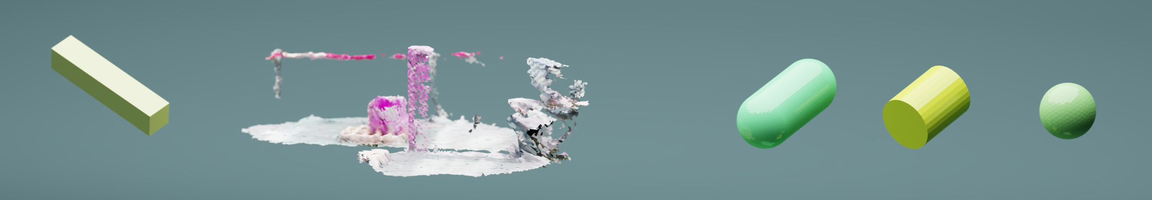
Five object types that are available in cuRobo’s WorldConfig are visualized, with Cuboid, Mesh, Capsule, Cylinder, and Sphere from left to right.
To use this world in a collision checker, we need to approximate some object types as cuRobo
currently only provides a collision checker for cuboids and meshes. Capsules, cylinders, and spheres
can be approximated to cuboids using curobo.geom.types.WorldConfig.create_obb_world,
# convert all objects into cuboids (oriented bounding boxes OBB)
cuboid_world = WorldConfig.create_obb_world(world_model)

cuboid_world.save_world_as_mesh("debug_collision_cuboid.obj")
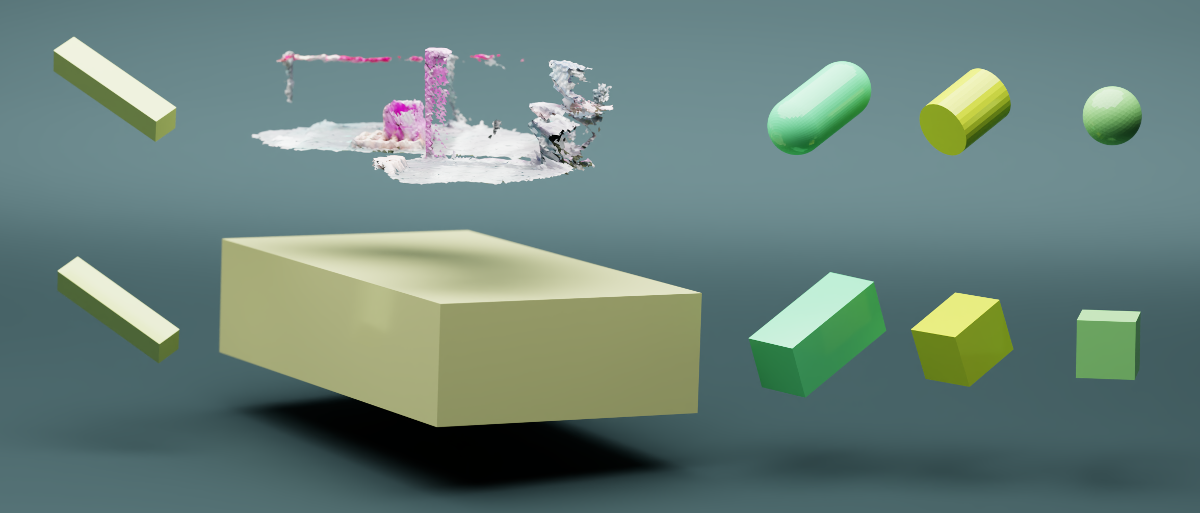
cuboid approximation of different object types are visulaized in the bottom row.
Alternatively, the objects can also be approximated as meshes, which are more accurate using,
# Keep cuboid objects as cuboids, nvblox as nvblox,  and convert all others to meshes.
collision_supported_world = WorldConfig.create_collision_support_world(world_model)
collision_support_world.save_world_as_mesh("debug_collision_mesh.obj")
Note
cuRobo’s cuboid collision checker is 4x faster than the mesh collision checker, so approximate objects to cuboids when possible to save compute time.
World Collision Checkers
There are four collision checkers available in cuRobo, all starting from an abstract base class
curobo.geom.sdf.world.WorldCollision. The cuboid collision checker is in
curobo.geom.sdf.world.WorldPrimitiveCollision which uses custom CUDA kernels to compute
collision and signed distance between query spheres and world cuboids. The mesh collision checker is
in curobo.geom.sdf.world_mesh.WorldMeshCollision, which uses a BVH traversal method to find
the closest point on a mesh given query spheres leveraging implementations available in NVIDIA Warp. cuRobo also provides a nvblox based collision checker
in curobo.geom.sdf.world_blox.WorldBloxCollision that can compute collisions with a list of
nvblox map instances that integrate camera depth images.
cuRobo also provides a voxel grid based
collision checker in curobo.geom.sdf.world_voxel.WorldVoxelCollision that can compute
collisions with respect to voxel grids that contain signed distance in each voxel. These voxel
grids can be filled with ESDF from other collision checkers to further speed up collision checking.
An example is provided in benchmarks/curobo_voxel_benchmark.py that stores a ESDF grid from
a world represented by cuboids.
cuRobo leverages python inheritance to combine collision checkers, where the nvblox collision checker inherits from the mesh collision checker and the mesh collision checker inherits from the cuboid collision checker.
Note
cuRobo does not provide mesh to mesh collision queries. Instead, collision checking is performed by approximating one object to spheres and performing closest point queries on meshes. cuRobo provides some approximation algorithms for converting meshes to spheres.
cuRobo’s collision checkers take as a input spheres which are of shape [batch, horizon, n, 4], where
n represents the number of spheres for one entity. cuRobo uses horizon to represent the trajectory
of a sphere, which is leveraged in cuRobo’s continuous collision checker. The output signed distance
will be of shape [batch, horizon, n], which can then be summed based on your use case. cuRobo
uses batch in two ways, (1) to parallelize across different rollouts such as in trajectory optimization, and
(2) to parallelize across different environments when available.
We can pass a world model to cuRobo’s collision checker and perform collision queries,
world_config = WorldCollisionConfig(tensor_args, world_model=collision_support_world)
world_ccheck = WorldMeshCollision(world_config)
world_ccheck.create_collision_cache(1)


new_mesh = Mesh(name="test_mesh", file_path=mesh_file, pose=[0, 0, 0, 1, 0, 0, 0])
world_ccheck.add_mesh(
   new_mesh,
   env_idx=0,
)
query_spheres = torch.zeros((1, 1, 2, 4), **vars(tensor_args))

out = world_ccheck.get_sphere_distance(query_spheres, collision_buffer,
act_distance,
weight)
out = out.view(-1)
Internally, each collision checker creates a tensorized object buffer on the GPU. Each object in the buffer will contain the object’s pose with respect to the robot’s base frame, geometry data, and a enable flag. This enable flag is used inside the collision kernels to know if the object is enabled for collision checking.
This object buffer is initialized based on the objects passed in through the world_model parameter in curobo.geom.sdf.world.WorldCollisionConfig. Optionally, you can set the buffer
size by passing a dictionary of number of objects per collision checker using the cache parameter
in curobo.geom.sdf.world.WorldCollisionConfig. cuRobo leverages this cache to load objects
later without having to recreate tensors, thereby not breaking any CUDAGraphs already built. This buffer is what enables the drag and drop interface in Isaac Sim, which is explained in Using with Isaac Sim page.
For example, you can create a cuboid object
buffer of 10 objects and mesh object buffer of 3 objects using cache={"obb":10, "mesh": 3}.
world_collision_config = WorldCollisionConfig(tensor_args, cache={"obb":10, "mesh": 3})
world_ccheck = WorldMeshCollision(world_collision_config)

new_cuboid = Cuboid(
  name="cube_1",
  pose=[0.0, 0.0, 0.0, 0.043, -0.471, 0.284, 0.834],
  dims=[0.2, 1.0, 0.2],
  color=[0.8, 0.0, 0.0, 1.0],
)


world_ccheck.add_cuboid(
   new_cuboid
)

new_mesh = Mesh(name="test_mesh", file_path=mesh_file, pose=[0, 0, 0, 1, 0, 0, 0])

world_ccheck.add_mesh(
   new_mesh,
)

query_spheres = torch.zeros((1, 1, 2, 4), **vars(tensor_args))

out = world_ccheck.get_sphere_distance(query_spheres, collision_buffer,
act_distance,
weight)
out = out.view(-1)
We can update the pose of objects that are in the cache by specifying the name of the object,
# update a cuboid obstacle pose
from curobo.types.math import Pose

new_pose = Pose.from_list([0,0,0.1,1,0,0,0], tensor_args=tensor_args)
world_ccheck.update_obstacle_pose(new_pose, name="cube_1")
We can toggle an object’s use in collision checking by using the enable_obstacle function,
world_ccheck.enable_obstacle("cube_1", enable=False)
Note
cuRobo’s signed distance queries return a positive value when the sphere is inside an obstacle or within activation distance. If outside this range, the distance value will be zero.
Batched Environments
cuRobo also provides batched world representation, where many worlds can be setup, and collision queries are mapped based on batch index of the spheres. We will look at a short python example below. A more thorough suite of examples are available in Batched Environments.
tensor_args = TensorDeviceType()
world_config_1 = WorldConfig(
   cuboid=[
      Cuboid(
            name="cube_env_1",
            pose=[0.0, 0.0, 0.0, 1.0, 0, 0, 0],
            dims=[0.2, 1.0, 0.2],
            color=[0.8, 0.0, 0.0, 1.0],
      )
   ]
)
world_config_2 = WorldConfig(
   cuboid=[
      Cuboid(
            name="cube_env_2",
            pose=[0.0, 0.0, 1.0, 1, 0, 0, 0],
            dims=[0.2, 1.0, 0.2],
            color=[0.8, 0.0, 0.0, 1.0],
      )
   ]
)

world_coll_config = WorldCollisionConfig(
   tensor_args, world_model=[world_config_1, world_config_2]
)

world_ccheck = WorldPrimitiveCollision(world_coll_config)

x_sph = torch.zeros((2, 1, 1, 4), device=tensor_args.device, dtype=tensor_args.dtype)
x_sph[..., 3] = 0.1

query_buffer = CollisionQueryBuffer.initialize_from_shape(
   x_sph.shape, tensor_args, world_ccheck.collision_types
)
act_distance = tensor_args.to_device([0.0])

weight = tensor_args.to_device([1])
querying sphere distance by default will only check with environment 0,
d = world_ccheck.get_sphere_distance(
   x_sph,
   query_buffer,
   weight,
   act_distance,
)

assert d[0] == 0.2 and d[1] == 0.2
passing an environment index, which contains the index of the collision environment per batch will query the spheres w.r.t. to the specified environment,
env_query_idx = torch.zeros((x_sph.shape[0]), device=tensor_args.device, dtype=torch.int32)
env_query_idx[1] = 1
d = world_ccheck.get_sphere_distance(
   x_sph, query_buffer, weight, act_distance, env_query_idx=env_query_idx
)

assert d[0] == 0.2 and d[1] == 0.0
Note that this environment is per batch and the query spheres shape is [batch, horizon, n, 4].
To perform collision checking with live depth images, refer to Using with Depth Camera tutorial.
Collision Checking Implementation
We want to be able to update the pose of obstacles without requiring additional post processing. To acheive this, we provide each obstacle type with a pose and project each query point to each obstacle’s local frame of reference to perform collision queries. While this can be slow on very large scenes as we would have to iterate over all objects, we found this to be better when working on less than 50 obstacles. This process is shown in the below flow chart. We leave using a fast world bvh (bounding volume hierarchy) for a later release (contributions welcome!).
We also implement a continuous collision checker that only requires a closest point function to implement. We dive into this algorithm in our technical report and only illustrate the computation flow below.
Collision checking process is illustrated.
Continuous collision checking process is illustrated.
Collision Metric
Our collision cost contains several configurable weights as listed in curobo.rollout.cost.primitive_collision_cost.PrimitiveCollisionCostConfig.
There are two main parameters, an activation distance \(\eta\) which determines how far away from a collision should the collision
cost needs to be computed, motivated by results from CHOMP. This is computed using the below
equation where \(d\) is the signed distance and is positive when in collision and negative outside collision,

The second parameter we use is the speed metric, which was also introduced in CHOMP. While in CHOMP, the speed metric was used with a discrete collision checker, cuRobo implements a continuous collision checker to account for thin obstacles. The speed metric is combined with this continuous collision checker to avoid obstacles in trajectory optimization. We show below the benefit of using the speed metric on a trajectory optimization problem. The left robot uses speed metric to push itself away from a thin wall while the right robot which does not have speed metric tries to rush through the collision as a way to reduce the overall cost incurred during trajectory optimization.
Geometry Approximation to Spheres
In manipulation tasks, we often need to grasp objects and relocate them to a different location. During the motion of the grasped object, we would need to avoid collisions between the attached object and the world. Since cuRobo’s collision checkers can only check between spheres and objects, we provide sphere generation techniques to approximate geometries to a set of spheres. These techniques require a large number of spheres (100+) to approximate complex geometry. We hence do not use these techniques to approximate robot geometry and rather use a tool in NVIDIA Isaac Sim to generate manually robots as described in Configuring a New Robot. However, the techniques can be used to approximate grasped objects during pick and place tasks.
Here is an example of fitting 500 spheres to approximate a capsule,
from curobo.geom.sphere_fit import SphereFitType
from curobo.geom.types import Capsule, WorldConfig

obstacle_capsule = Capsule(
   name="capsule",
   radius=0.2,
   base=[0, 0, 0],
   tip=[0, 0, 0.5],
   pose=[0.0, 5, 0.0, 0.043, -0.471, 0.284, 0.834],
   color=[0, 1.0, 0, 1.0],
)

sph = obstacle_capsule.get_bounding_spheres(n_spheres=500)

WorldConfig(spheres=sph).save_world_as_mesh("bounding_spheres.obj")

WorldConfig(capsule=[obstacle_capsule]).save_world_as_mesh("capsule.obj")
cuRobo provides five different methods to fit spheres to geometry as listed in
curobo.geom.sphere_fit.SphereFitType. The fit types leverage voxelization of geometry and
surface sampling to approximate a geometry. In short,
SAMPLE_SURFACEsamples the surface of the mesh to approximate geometry.VOXEL_SURFACEvoxelizes the volume and returns voxel positions that are intersecting with surface.VOXEL_VOLUME_INSIDEvoxelizes the volume and returns voxel positions that are inside the surface of the geometry.VOXEL_VOLUMEvoxelizes the volume and returns all ocupioed voxel positions.VOXEL_VOLUME_SAMPLE_SURFACEvoxelizes the volume and returns voxel positions that are inside the surface, along with surface sampled positions.
The effect of each fit type on YCB objects is visualized below,
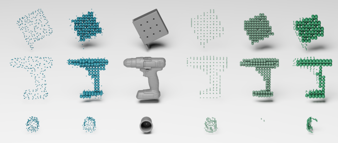
From left to right: SAMPLE_SURFACE, VOXEL_VOLUME_SAMPLE_SURFACE, Mesh, VOXEL_SURFACE, VOXEL_VOLUME_INSIDE, VOXEL_VOLUME.